WSwavelet User Guide

Nilotpal Sanyal

September 2026

Introduction and overview

What problem does WSwavelet solve?

Wavelet denoising is useful when a signal contains sharp peaks, abrupt transitions, localized features, or rapid oscillations. An orthogonal discrete wavelet transform represents such a signal using a small set of coarse scaling coefficients and detail coefficients at multiple resolutions. The observed detail coefficients are noisy and are often sparse: most are close to zero while a smaller number carry important signal features.

WSwavelet implements a Bayesian shrinkage rule for this setting. Its prior has an explicit point mass at zero and a bounded continuous slab formed by a mixture of two normalized densities:

1. a concentrated, compactly supported Wendland-type density; and
2. a more dispersed semicircle density.

The relative contribution of the two slab components can vary with resolution through a low-dimensional empirical-Bayes trend. The package provides Gaussian and Laplace coefficientwise likelihoods. The Gaussian version is the primary practical specification; the Laplace version is an alternative working-likelihood analysis for sensitivity to non-Gaussian observation errors.

WSwavelet in one picture

For an input signal y, the main function follows this sequence:

1. Apply an orthogonal discrete wavelet transform.
2. Estimate the noise standard deviation by a robust high-frequency MAD rule, unless a known value is supplied.
3. Construct a level-specific support scale and spike probability.
4. Fit the slab mixture weight by bounded empirical-Bayes optimization.
5. Replace each detail coefficient by its posterior mean.
6. Reconstruct the signal by the inverse discrete wavelet transform.

The scaling coefficients are retained without shrinkage. The package requires a finite input vector of dyadic length, such as 128, 256, or 1024.

Installation and first example

Installation

Install the wavelet dependency and then install the WSwavelet source archive:

install.packages("wavethresh")
install.packages("WSwavelet_0.1.0.tar.gz", repos = NULL, type = "source")

Load the package:

library(WSwavelet)

A reproducible synthetic signal

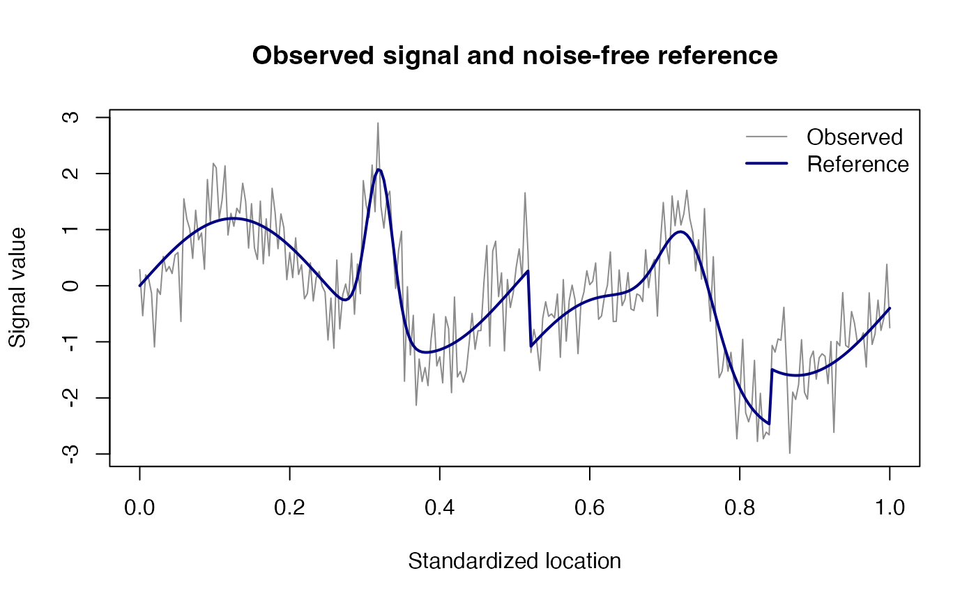
The package does not impose a particular signal-generating model. The following example combines a smooth oscillation with a narrow peak and two localized transitions, giving the denoiser several types of structure to recover.

set.seed(2026)

n <- 256L
x <- seq(0, 1, length.out = n)

demo_signal <- function(x) {
  1.2 * sin(4 * pi * x) +
    3.0 * exp(-((x - 0.32) / 0.025)^2) +
    2.0 * exp(-((x - 0.73) / 0.05)^2) -
    1.4 * (x > 0.52) +
    1.0 * (x > 0.84)
}

truth <- demo_signal(x)
y <- truth + rnorm(n, sd = 0.55)

plot(
  x, y, type = "l", col = "grey55",
  xlab = "Standardized location", ylab = "Signal value",
  main = "Observed signal and noise-free reference"
)
lines(x, truth, col = "navy", lwd = 2)
legend(
  "topright",
  legend = c("Observed", "Reference"),
  col = c("grey55", "navy"), lty = 1, lwd = c(1, 2),
  bty = "n"
)

Fitting the primary Gaussian version

The main function is wswavelet(). For a quick vignette run, the example uses a short wavelet filter and 24 quadrature nodes. For production analyses, the default filter and quadrature settings can be used or increased after checking computational cost.

fit_g <- wswavelet(
  y = y,
  likelihood = "gaussian",
  filter.number = 2L,
  family = "DaubExPhase",
  bc = "periodic",
  quadrature_n = 24L
)

plot(
  x, y, type = "l", col = "grey60",
  xlab = "Standardized location", ylab = "Signal value",
  main = "WS-Gaussian reconstruction"
)
lines(x, truth, col = "navy", lwd = 2)
lines(x, fit_g$estimate, col = "firebrick", lwd = 2)
legend(
  "topright",
  legend = c("Observed", "Reference", "WS-Gaussian"),
  col = c("grey60", "navy", "firebrick"),
  lty = 1, lwd = c(1, 2, 2), bty = "n"
)

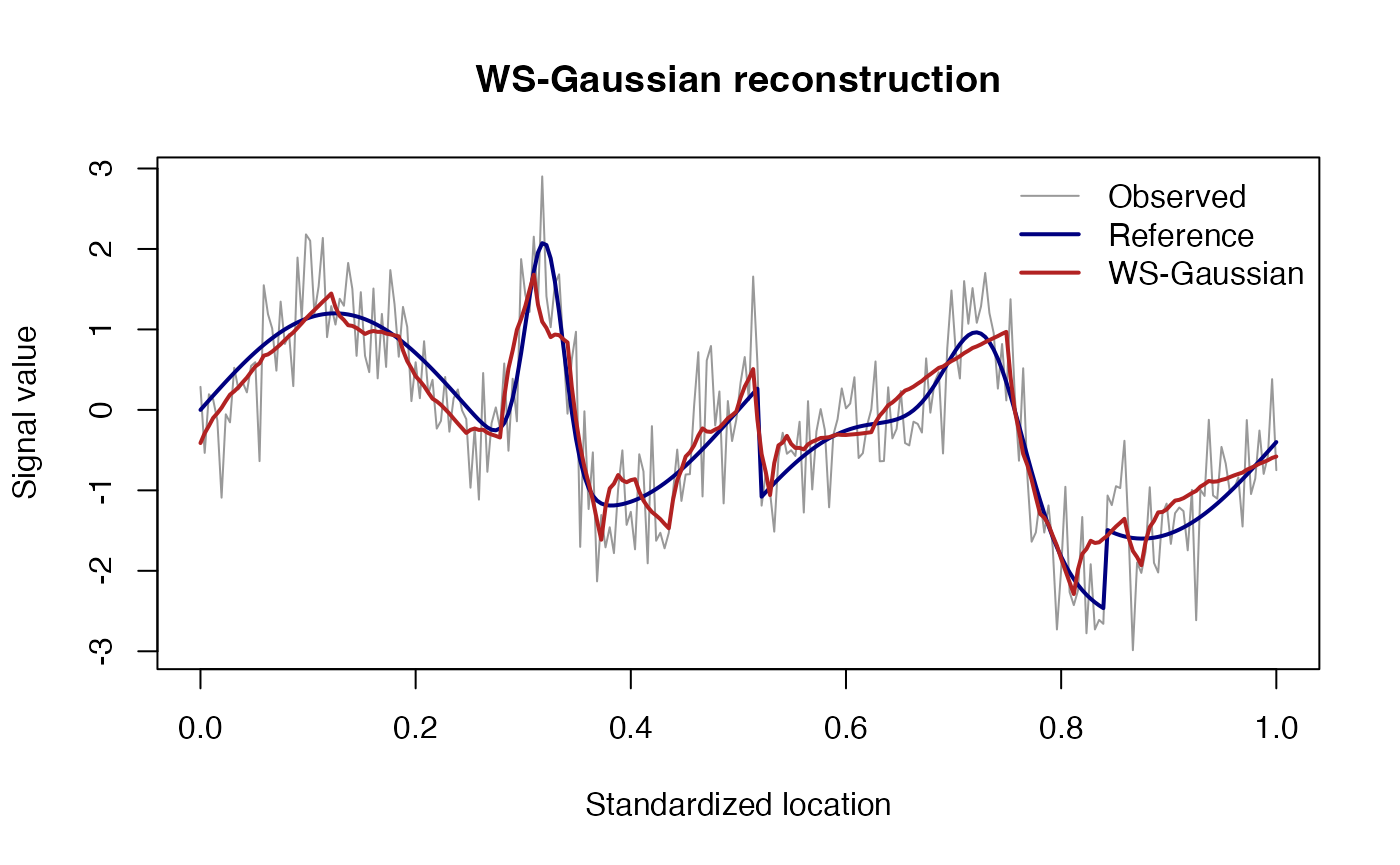
The fitted signal is stored in fit_g$estimate. Important fitted quantities are:

fit_g$sigma_hat
#> [1] 0.5958579
fit_g$eta_hat
#> [1] -12 -12
fit_g$optimization$convergence
#> [1] 0

The level summary gives the resolution-specific hyperparameters and average posterior component probabilities:

head(
  fit_g$level_summary[, c(
    "level", "coefficients", "spike_probability", "beta", "omega",
    "mean_p0", "mean_pW", "mean_pS"
  )]
)
#>   level coefficients spike_probability     beta        omega      mean_p0
#> 0     0            1         0.8105354 4.180959 6.144175e-06 1.815194e-09
#> 1     1            2         0.9284007 8.109933 1.106524e-06 8.746042e-08
#> 2     2            4         0.9641032 6.232857 1.992767e-07 2.587512e-01
#> 3     3            8         0.9789878 4.363048 3.588820e-08 4.975558e-01
#> 4     4           16         0.9864345 3.537500 6.463190e-09 8.689578e-01
#> 5     5           32         0.9906295 2.427249 1.163971e-09 9.582905e-01
#>        mean_pW    mean_pS
#> 0 1.607347e-07 0.99999984
#> 1 3.597331e-07 0.99999955
#> 2 4.669356e-08 0.74124880
#> 3 4.550149e-09 0.50244424
#> 4 1.672502e-10 0.13104221
#> 5 1.663571e-11 0.04170949

The fitted detail-level objects contain the observed coefficients, posterior means, posterior component probabilities, component-specific means, support scales, and numerical fallback counts:

names(fit_g$detail[[1L]])
#>  [1] "level"                 "observed"              "estimate"             
#>  [4] "posterior_probability" "component_mean"        "component_log_m0"     
#>  [7] "beta"                  "spike_probability"     "omega"                
#> [10] "quadrature_fallbacks"

Statistical model

Wavelet-domain observation model

Let $d_{j,k}$ denote an observed detail coefficient at level j, and let $\theta_{j,k}$ denote its unknown signal coefficient. The coefficientwise working model is

$$d_{j,k} = \theta_{j,k} + \epsilon_{j,k}^{*}.$$

For the Gaussian version,

$$\epsilon_{j,k}^{*}\sim N(0,\sigma^2), \qquad L_N(d\mid\theta,\sigma^2) =\frac{1}{\sqrt{2\pi\sigma^2}} \exp\left\{-\frac{(d-\theta)^2}{2\sigma^2}\right\}.$$

The implementation uses the Laplace likelihood as an alternative working specification:

$$L_L(d\mid\theta,\lambda) =\frac{a}{2}\exp\{-a|d-\theta|\}, \qquad a=\sqrt{2\lambda}.$$

When laplace_rate = NULL, the main fitting function sets $\widehat{\lambda}=1/(2\widehat{\sigma}^2)$ once and keeps it fixed during empirical-Bayes optimization.

Wendland and semicircle slab densities

The standardized Wendland-type density is

$$K_W(u)=\frac{3}{2}(1-|u|)^4(1+4|u|)I(|u|<1),$$

and the standardized semicircle density is

$$K_S(u)=\frac{2}{\pi}\sqrt{1-u^2}I(|u|<1).$$

For a positive support scale beta, the corresponding coefficient-scale densities are

$$g_W(\theta;\beta)=\frac{1}{\beta}K_W(\theta/\beta), \qquad g_S(\theta;\beta)=\frac{1}{\beta}K_S(\theta/\beta).$$

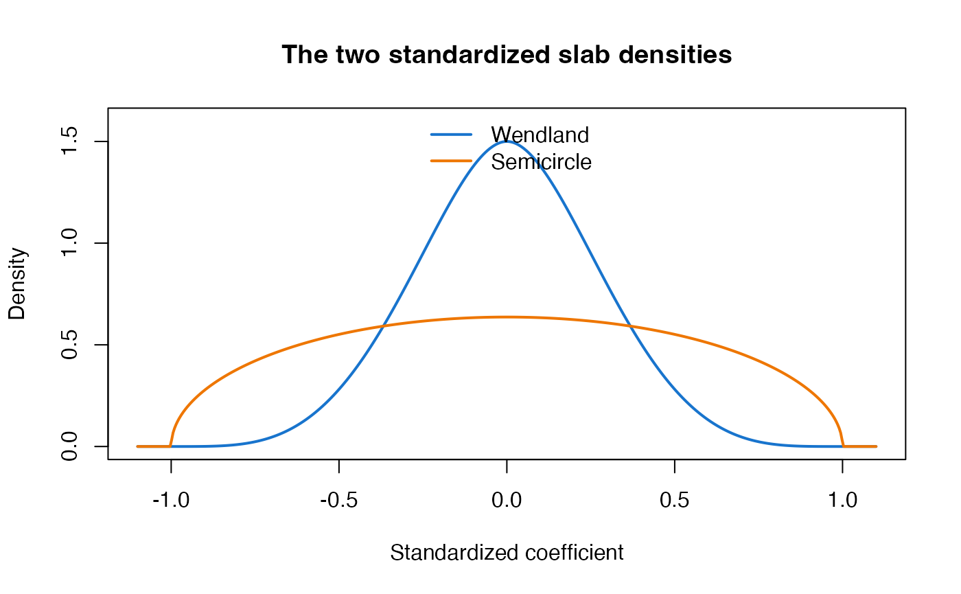
Both slab densities are symmetric and supported on $[-\beta,\beta]$. The Wendland component is more concentrated near zero, whereas the semicircle component is more dispersed.

The densities can be evaluated directly:

u <- seq(-1.1, 1.1, length.out = 501L)
plot(
  u, wendland_kernel(u), type = "l", lwd = 2, col = "dodgerblue3",
  ylim = c(0, 1.6), xlab = "Standardized coefficient",
  ylab = "Density", main = "The two standardized slab densities"
)
lines(u, semicircle_kernel(u), lwd = 2, col = "darkorange2")
legend(
  "top", legend = c("Wendland", "Semicircle"),
  col = c("dodgerblue3", "darkorange2"), lty = 1, lwd = 2,
  bty = "n"
)

Spike-and-slab prior

At level j, the prior is

$$\theta_{j,k}\sim \pi_j\delta_0+ (1-\pi_j) \left\{\omega_jg_W(\theta;\beta_j) +(1-\omega_j)g_S(\theta;\beta_j)\right\}.$$

The three prior component probabilities are therefore

$$\Pr(Z_{j,k}=0)=\pi_j,\qquad \Pr(Z_{j,k}=W)=(1-\pi_j)\omega_j,\qquad \Pr(Z_{j,k}=S)=(1-\pi_j)(1-\omega_j).$$

The spike probability increases with resolution according to

$$\pi_j=1-(j-j_0+\ell)^{-\gamma},$$

where ell is spike_offset and gamma is spike_gamma. This expresses the working assumption that finer-scale coefficients are more likely to be noise.

Resolution-dependent slab weights

For the adaptive model, define

$$t_j=\frac{j-j_0}{J-1-j_0}, \qquad \omega_j(\eta)= \operatorname{logit}^{-1}(\eta_0+\eta_1t_j).$$

The two empirical-Bayes parameters eta_0 and eta_1 control the baseline Wendland contribution and its change across resolution. Setting omega_model = “constant” estimates only a common weight. Supplying fixed_omega = 0 or fixed_omega = 1 evaluates the semicircle-only or Wendland-only endpoint, respectively.

Data-adaptive support scale

The initial support scale at level j is

$$\widehat{\beta}^{(0)}_j =\max\left\{\widehat{\sigma}, Q_\kappa\left(\{|d_{j,k}|: k\in\mathcal K_j\}\right)\right\},$$

where kappa is beta_quantile. The implementation then applies the positive floor

$$\beta_{\min}=\epsilon_\beta s_\beta,\qquad s_\beta=\max\left\{1,\widehat{\sigma}, \max_{j,k}|d_{j,k}|\right\}, \qquad \widehat{\beta}_j=\max\{\widehat{\beta}^{(0)}_j,\beta_{\min}\}.$$

This is a data-adaptive truncation-scale rule, not a formal guarantee that future or unobserved coefficients lie inside the fitted support.

Posterior shrinkage

The coefficient-level posterior

The function level_posterior() applies the posterior calculation to a vector of coefficients at one level. For c in $\{W,S\}$, define the component moments

$$M_{r,c,j}(d) =\int_{-\beta_j}^{\beta_j} \theta^r g_c(\theta;\beta_j)L(d\mid\theta)\,d\theta, \qquad r\in\{0,1\}.$$

The marginal density of d under the full prior is

$$D_j(d) =\pi_jL(d\mid0) +(1-\pi_j) \left\{\omega_jM_{0,W,j}(d) +(1-\omega_j)M_{0,S,j}(d)\right\}.$$

The posterior component probabilities are

$$p_{0,j}(d)=\frac{\pi_jL(d\mid0)}{D_j(d)},$$

$$p_{W,j}(d)= \frac{(1-\pi_j)\omega_jM_{0,W,j}(d)}{D_j(d)}, \qquad p_{S,j}(d)= \frac{(1-\pi_j)(1-\omega_j)M_{0,S,j}(d)}{D_j(d)}.$$

Conditional on the two continuous components,

$$\mu_{W,j}(d)=\frac{M_{1,W,j}(d)}{M_{0,W,j}(d)}, \qquad \mu_{S,j}(d)=\frac{M_{1,S,j}(d)}{M_{0,S,j}(d)}.$$

Under squared-error loss, the posterior-mean shrinkage estimate is

$$\delta_j(d) =p_{W,j}(d)\mu_{W,j}(d) +p_{S,j}(d)\mu_{S,j}(d).$$

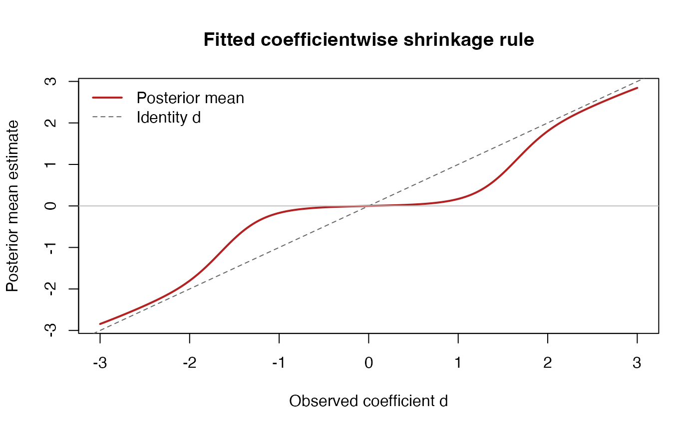
The spike contributes zero to the posterior mean. Thus, a positive spike probability does not by itself force an exact zero estimate; it expresses posterior evidence for the point-mass component, while the posterior mean is generally a continuous shrinkage rule.

Inspecting one shrinkage curve

evaluate_shrinkage_curve() evaluates the fitted rule over hypothetical coefficient values. level_index is the position of the level in fit$detail, not necessarily the numerical wavelet-level label.

curve_g <- evaluate_shrinkage_curve(
  fit_g,
  level_index = 1L,
  d_grid = seq(-3, 3, length.out = 301L)
)

plot(
  curve_g$d, curve_g$estimate, type = "l", lwd = 2,
  col = "firebrick", xlab = "Observed coefficient d",
  ylab = "Posterior mean estimate",
  main = "Fitted coefficientwise shrinkage rule"
)
abline(0, 1, lty = 2, col = "grey40")
abline(h = 0, col = "grey75")
legend(
  "topleft",
  legend = c("Posterior mean", "Identity d"),
  col = c("firebrick", "grey40"), lty = c(1, 2), lwd = c(2, 1),
  bty = "n"
)

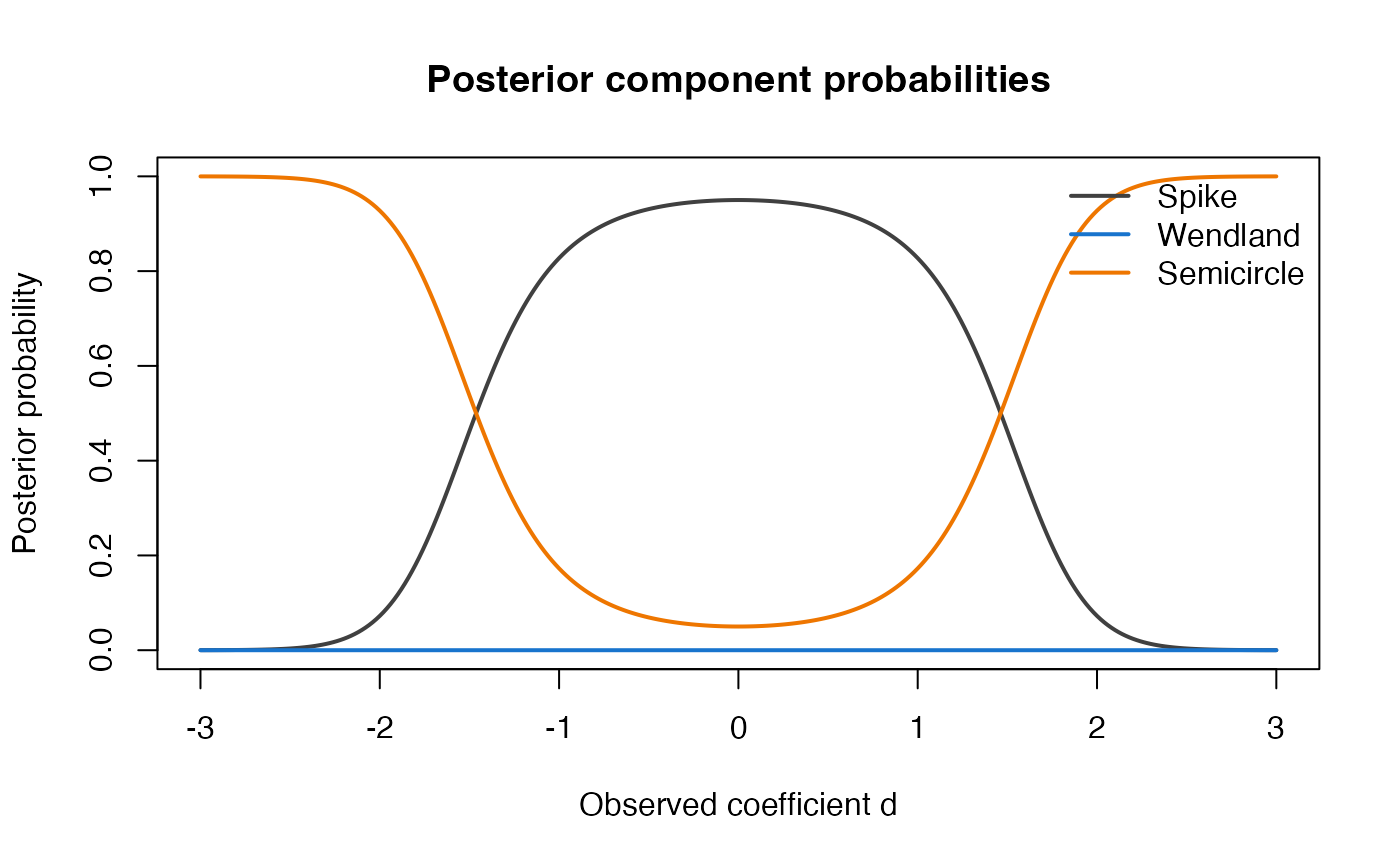
The posterior component probabilities can be inspected on the same grid:

matplot(
  curve_g$d,
  curve_g[, c("posterior_spike", "posterior_wendland",
              "posterior_semicircle")],
  type = "l", lty = 1, lwd = 2,
  col = c("grey25", "dodgerblue3", "darkorange2"),
  xlab = "Observed coefficient d", ylab = "Posterior probability",
  main = "Posterior component probabilities"
)
legend(
  "topright",
  legend = c("Spike", "Wendland", "Semicircle"),
  col = c("grey25", "dodgerblue3", "darkorange2"),
  lty = 1, lwd = 2, bty = "n"
)

Using level_posterior() independently

The low-level posterior function is useful when a user already has wavelet coefficients and wants posterior quantities without fitting a complete signal. For example, the following uses the first fitted level’s parameters:

level_fit <- fit_g$detail[[1L]]

post <- level_posterior(
  d = c(-1, 0, 1),
  pi_j = level_fit$spike_probability,
  omega_j = level_fit$omega,
  beta_j = level_fit$beta,
  sigma = fit_g$sigma_hat,
  likelihood = fit_g$likelihood,
  laplace_rate = fit_g$laplace_rate_hat,
  quadrature_n = fit_g$settings$quadrature_n,
  use_exact_wendland = fit_g$settings$use_exact_wendland
)

post$posterior_mean
#> [1] -1.686853e-01  6.040471e-18  1.686853e-01
post$probability
#>          spike     wendland semicircle
#> [1,] 0.8274089 1.665236e-06 0.17258945
#> [2,] 0.9500170 6.374974e-07 0.04998237
#> [3,] 0.8274089 1.665236e-06 0.17258945

Likelihood options and model variants

Laplace working likelihood

The Laplace version is fitted by setting likelihood = “laplace”:

fit_l <- wswavelet(
  y,
  likelihood = "laplace",
  filter.number = 2L,
  family = "DaubExPhase",
  bc = "periodic",
  quadrature_n = 24L
)

The default rate is computed once from the robust noise estimate and held fixed. For Laplace fits, the Wendland component has a finite-sum expression with a numerical fallback; the semicircle component is evaluated by Gauss-Legendre quadrature after a change of variables that handles the square-root endpoint behavior. Set use_exact_wendland = FALSE to use quadrature for the Wendland component as well.

The Laplace option should be interpreted as an alternative working likelihood, not as a guarantee of uniformly improved performance. Its usefulness depends on the actual error distribution and on the signal and SNR regime.

Constant and endpoint slab specifications

The default adaptive model estimates both the intercept and resolution trend in the logistic Wendland weight. For component or sensitivity analyses, the following alternatives are available:

# One common empirical-Bayes mixture weight:
fit_constant <- wswavelet(
  y, likelihood = "gaussian", omega_model = "constant"
)

# Wendland-only endpoint:
fit_wendland <- wswavelet(
  y, likelihood = "gaussian", fixed_omega = 1
)

# Semicircle-only endpoint:
fit_semicircle <- wswavelet(
  y, likelihood = "gaussian", fixed_omega = 0
)

These endpoint fits are useful for understanding how the two slab shapes contribute to the complete model. They are not separate thresholding methods.

Independent utility functions

Estimating the noise scale

estimate_noise_sd() can be used independently when a wavelet object has already been constructed:

wavelet_object <- wavethresh::wd(
  y,
  filter.number = 2L,
  family = "DaubExPhase",
  type = "wavelet",
  bc = "periodic",
  verbose = FALSE
)
detail_levels <- 0:(wavethresh::nlevelsWT(wavelet_object) - 1L)

estimate_noise_sd(
  wavelet_object,
  detail_levels = detail_levels,
  mad_levels = 1L
)
#> [1] 0.5958579

Unless a known supplied_sd is provided, the estimator is

$$\widehat{\sigma} =\frac{\operatorname{median} \left(|d-\operatorname{median}(d)|\right)}{0.6745},$$

computed from the finest selected detail levels. If the result is not positive and finite, the implementation pools up to three of the finest available levels and then applies a strictly positive machine-scale fallback if needed.

Numerical checks

ws_numerical_checks() evaluates a fixed grid for Gaussian and Laplace likelihoods and for endpoint and interior values of the spike probability and Wendland weight:

checks <- ws_numerical_checks(quadrature_n = 32L)
head(
  checks[, c(
    "likelihood", "pi", "omega", "max_oddness_error",
    "min_first_difference", "max_support_excess", "all_finite"
  )]
)
#>   likelihood  pi omega max_oddness_error min_first_difference
#> 1   gaussian 0.0     0      6.661338e-15         9.141978e-04
#> 2    laplace 0.0     0      2.664535e-15        -8.881784e-16
#> 3   gaussian 0.5     0      6.661338e-15         9.142390e-04
#> 4    laplace 0.5     0      1.554312e-15        -1.554312e-15
#> 5   gaussian 1.0     0      0.000000e+00         0.000000e+00
#> 6    laplace 1.0     0      0.000000e+00         0.000000e+00
#>   max_support_excess all_finite
#> 1                  0       TRUE
#> 2                  0       TRUE
#> 3                  0       TRUE
#> 4                  0       TRUE
#> 5                  0       TRUE
#> 6                  0       TRUE

The checks include:

• oddness of the shrinkage map, $\delta(-d)=-\delta(d)$;
• boundedness by the fitted support, $|\delta(d)|\leq\beta$;
• finite posterior means;
• exact handling of $\pi=0$ and $\pi=1$; and
• nondecreasing behavior on the evaluation grid for the fixed Gaussian rule.

The routine is a diagnostic rather than a formal proof. Its numerical errors should be interpreted relative to the quadrature order and floating-point precision.

Practical guidance and troubleshooting

Choosing the likelihood

Use the Gaussian version as the primary default when the observation errors are reasonably close to Gaussian or when computational efficiency is a priority. The Laplace option is useful as a robustness-oriented sensitivity analysis when heavier-tailed or more sharply peaked errors are plausible.

Choosing the quadrature order

The default quadrature_n = 48L is intended to provide a stable general-purpose calculation. Lower values can make exploratory analyses faster; higher values may be appropriate for numerical validation or difficult parameter regimes. The returned diagnostics record the number of exact Wendland calculations that required numerical fallback.

Input length and boundaries

The current implementation requires a finite signal vector of dyadic length. It uses the boundary convention accepted by wavethresh, with bc = “periodic” by default. If the original record is not dyadic, users should document their padding or extension rule before calling the package and truncate any reconstructed padded values before application-level interpretation.

Interpreting the support scale

The fitted beta_j is a data-adaptive truncation scale. It is not a formal estimator of an unknown physical support and does not guarantee that future coefficients remain inside the fitted interval. The quantile rule reduces sensitivity to isolated outliers compared with a maximum-based rule.

Reproducibility

The fitting procedure itself is deterministic for fixed inputs and settings. For reproducible simulations, set the seed when generating the noisy signal, record the package version, save the complete fitted object, and report the wavelet family, boundary convention, quadrature order, noise-scale rule, and likelihood.

Citation

Please cite the methodological paper when using WSwavelet:

Sanyal, N. (2026). Resolution-Adaptive Compact-Support Priors for Bayesian Wavelet Denoising: A Wendland-Semicircle Slab Mixture for Low-SNR Signal Recovery. Axioms, 15(9), 678. https://doi.org/10.3390/axioms15090678.