BHMSMAfMRI User Guide
Nilotpal Sanyal
January 22, 2026
Source:vignettes/BHMSMAfMRIvignette.Rmd
BHMSMAfMRIvignette.RmdWelcome to BHMSMAfMRI, an R package to analyze functional MRI (fMRI) data, or other multiscale data. This manual shows how the BHMSMAfMRI package functions are used to analyze fMRI data and should be helpful for the first-time user. In Section @ref(secintro), we give a short introduction and non-mathematical overview of the methodology, and in Section @ref(secuse), we discuss the package functions in a systematic way and apply them to analyze a simulated fMRI dataset.
Introduction and overview
The BHMSMAfMRI package performs Bayesian hierarchical multi-subject multiscale analysis (BHMSMA) of fMRI data (Sanyal and Ferreira 2012), or other multiscale data. Though fMRI data is generally 3D, currently BHMSMAfMRI considers analysis of 2D slices only.
The main features of the BHMSMA method are that:
- it takes into account both the temporal and the spatial information contained in the fMRI data,
- it performs multi-subject analysis and borrows strength across subjects for precise estimation of the effect sizes (i.e., brain activations), and provides a straightforward way to obtain group activation map, and
- it does not use Markov Chain Monte Carlo (MCMC) simulation and is fast.
BHMSMA models the temporal variation present in the fMRI data through a general linear model (GLM) and then considers discrete wavelet transform of the standardized regression coefficients for harnessing the spatial information. In the wavelet domain, each wavelet coefficient is assigned a mixture prior that is a combination of a Gaussian density and a point mass at zero. This prior specification takes into account the sparsity of the wavelet coefficients. For the mixture probabilities BHMSMA considers a prior that depends on few hyperparameters. Inference is carried out by an empirical Bayes methodology without using MCMC methods. The inference uses approximation of one-dimensional integrals only. The posterior mean of the regression coefficients are obtained by using the posterior mean of the wavelet coefficients in the inverse discrete wavelet transform. Further, the posterior wavelet coefficients are averaged over subjects and used in the inverse discrete wavelet transform to obtain posterior group estimate of the regression coefficients. Posterior uncertainty is assessed based on simulations from the posterior distribution of the regression coefficients.
The BHMSMAfMRI package fits the BHMSMA model to the fMRI data and provides estimates of the hyperparameters along with their standard error, posterior mean of the wavelet coefficients, posterior mean of the regression coefficients, samples from the posterior distribution of the regression coefficients and posterior group estimate of the regression coefficients. The posterior samples can be used to compute the estimates of posterior standard deviation and posterior probability maps.
Use of package functions with examples
In this section we illustrate the use of the package functions. We assume that prior to applying our methodology, the fMRI data have been preprocessed for necessary corrections like realignment or motion correction, slice-timing correction, coregistration with anatomical image and normalization. However, the data must not be spatially filtered before applying BHMSMA, because our approach is to include the spatial information into modeling instead of filtering it out. Preprocessing can be perfomed by using available softwares/packages like SPM (Friston et al. 2007), BrainVoyager (Goebel, Esposito, and Formisano 2006), AFNI (Cox 1996), and FSL (Smith et al. 2004). In the following subsections, we show the use of the package functions in a systematic way.
The main function BHMSMA
BHMSMA is the main function of the
BHMSMAfMRI package. BHMSMA accepts fMRI
data as a 4D array. The data can be imported from various image files by
the readfmridata function. BHMSMA successively
calls the following functions to perform the whole analysis —
glmcoef to obtain regression coefficient map of the
regressor of interest, waveletcoef to perform 2D wavelet
transformation of the regression coefficient map,
hyperparamest to obtain estimates of the BHMSMA model
hyperparameters, postmixprob to obtain estimates of the
mixture probabilities that define posterior distribution of the wavelet
coefficients, postwaveletcoef to obtain the posterior
estimates of the wavelet coefficients and finally
postglmcoef to obtain the posterior smoothed version of the
regression coefficient map. If true coefficients are given,
BHMSMA also returns mean squared error (MSE) estimates.
Here is a quick look at the usage and outputs of the function.
library(BHMSMAfMRI)
BHMSMAmulti <- BHMSMA(n, grid, data, designmat, k, "multi", truecoef)
names(BHMSMAmulti)
[1] "GLMCoefStandardized"      "GLMCoefSE"
[3] "WaveletCoefficientMatrix" "hyperparam"
[5] "hyperparamVar"            "posteriorMixProb"
[7] "Waveletcoefposterior"     "GLMcoefposterior"
The dimension of data is
c(n,grid,grid,ntime) where n is the number of
sujects, grid^2 is the total number of voxels in the data
and ntime is the length of time-series for each voxel. The
argument k selects the regressor of interest from the
design matrix designmat which can have multiple regressor
columns. Following sections break down the whole analysis shown above by
showing specific uses and outputs of all the above functions and several
others of the BHMSMAfMRI package.
Reading fMRI Data: readfmridata
The function readfmridata can read fMRI data file(s)
stored in ANALYZE format (.img/.hdr files), NIFTI format (.img/.hdr
files or .nii files) or AFNI format (.BRIK/.HEAD files). The reading of
the fMRI data files is done using R package oro.nifti
(Whitcher, Schmid, and Thornton 2011),
which is loaded when BHMSMAfMRI package is loaded.
For illustration, we consider a simulated fMRI dataset stored in
ANALYZE format and provided within the BHMSMAfMRI
package. The dataset contains noisy fMRI data collected over a
grid of a single axial brain slice and at 9 timepoints for 3 subjects.
The following code illustrates how the function
readfmridata can be used to import the data from the image
files. The simulated dataset is extracted in the directory
fmridata within the R temporary folder.
##
##  Welcome! Thanks for trying BHMSMAfMRI.
##
##  Website: https://nilotpalsanyal.github.io/BHMSMAfMRI/
##  Bug report: https://github.com/nilotpalsanyal/BHMSMAfMRI/issues
fpath <- system.file("extdata", package="BHMSMAfMRI")
untar(paste0(fpath,"/fmridata.tar"), exdir=tempdir())
n <- 3
grid <- 32
ntime <- 9
data <- array(dim=c(n,grid,grid,ntime))
for(subject in 1:n)
{
  directory <- paste0(tempdir(),"/fmridata","/s0",subject,"/")
  a <- readfmridata(directory, format="Analyze",
  prefix=paste0("s0",subject,"_t"), nimages=ntime, dim.image=c(grid,grid,1))
  data[subject,,,] <- a[,,1,]
}
dim(a)
## [1] 32 32 1 9The above code reads all the data files for all subjects into a 4D
array data. For each subject, the data were generated by
adding Gaussian random noise to the true regression coefficient image
with activation in 3 regions. The positions of 2 activation regions were
varied across subject. The underlying design was a block design. The
true regression coefficient images and the design matrix are also
included in the package and can be read as follows.
## [1] "grid" "nsubject" "TrueCoeff" "DesignMatrix"
truecoef <- fmridata$TrueCoeff
designmat <- fmridata$DesignMatrix
dim(truecoef)
## [1] 3 32 32
dim(designmat)## [1] 9 2Now, we have truecoef which is an array of dimension (3,
32, 32) containing the true regression coefficients, data
which is an array of dimension (3, 32, 32, 9) containing time series of
noisy observations for all the subjects and designmat which
is the design matrix used to generate the data. Note that, the R package
neuRosim (Welvaert et al.
2011) can be used to generate fMRI data.
par(mfrow=c(1,n), cex=1)
for(subject in 1:n)
  image(truecoef[subject,,], main=paste0("Subject ",subject),
         col=heat.colors(8))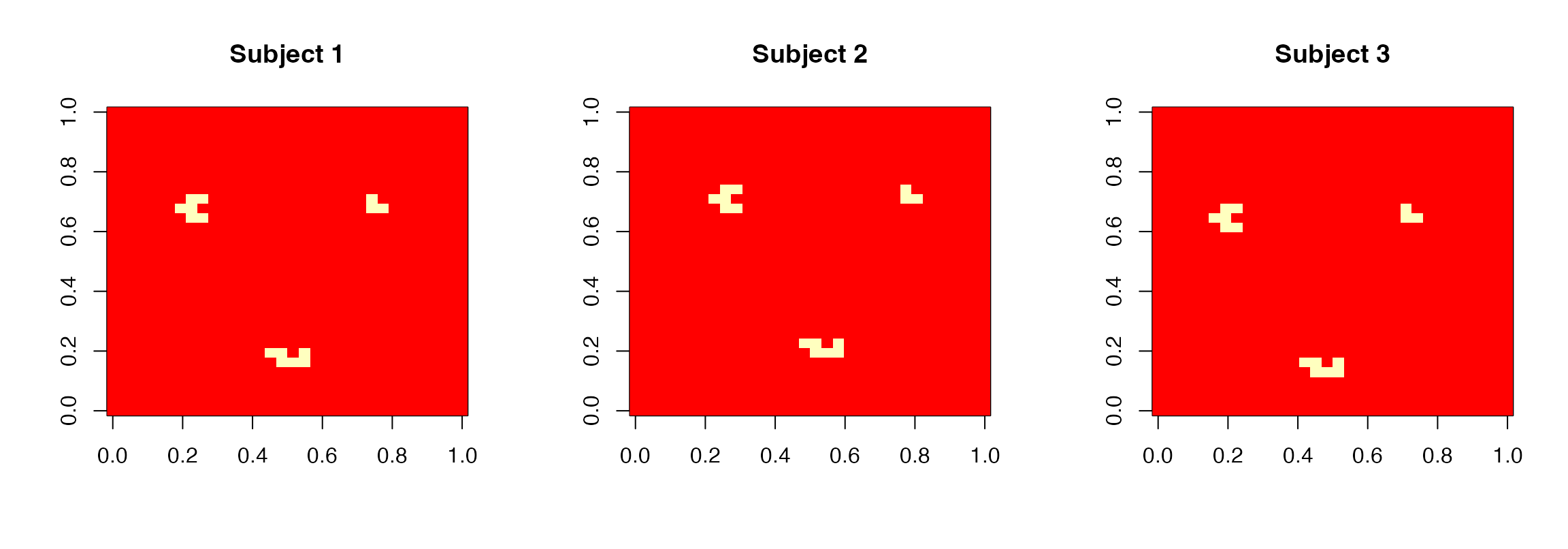
True regression coefficient images for the 3 subjects
Temporal modeling through GLM: glmcoef
Now, we fit a general linear model to the time series of each voxel
and obtain the estimated regression coefficients for all the regressors
included in designmat by using the function
glmcoef as follows.
## [1] "GLMCoefStandardized" "GLMCoefSE"
dim(glmmap$GLMCoefStandardized)## [1] 3 32 32 2
dim(glmmap$GLMCoefSE)## [1] 3 32 32 2The output glmmap contains the estimated standardized
regression coefficients and their standard error estimates. From now on,
we focus on the
2
regressor as the regressor of interest. Figure @ref(fig:GLMCoef),
obtained by the following code, shows the images of its standardized
regression coefficients estimates for the 3 subjects.
k <- 2
par(mfrow=c(1,n), cex=1)
for(subject in 1:n)
  image(abs(glmmap$GLMCoefStandardized[subject,,,k]), col=heat.colors(8),
         zlim=c(0,6), main=paste0("Subject ",subject))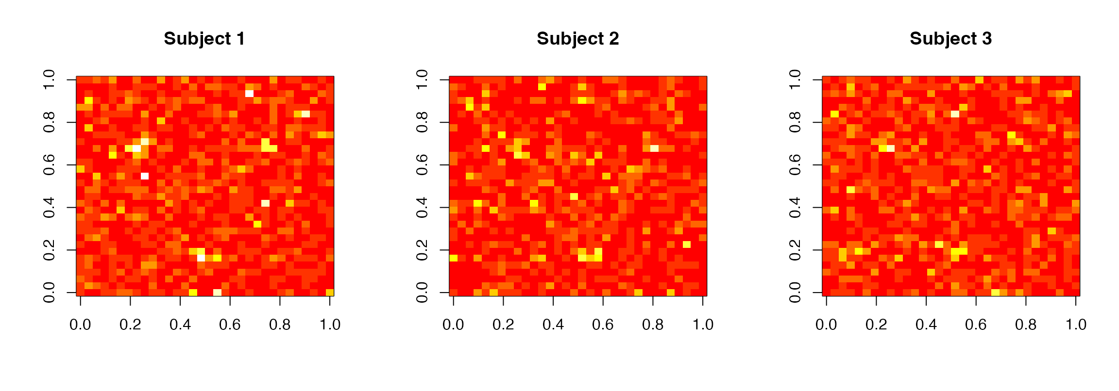
Standardized regression coefficient estimates images for the second regressor for all subjects
Wavelet transform of the GLM coefficients:
waveletcoef
Next, we apply the discrete wavelet transform to the standardized regression coefficient images of each subject. The wavelet transformation is performed by the using the R package wavethresh (Nason 2013), which is loaded when BHMSMAfMRI package is loaded.
The function waveletcoef returns the wavelet
coefficients for the selected regressor for all the subjects as a
matrix. Below it is illustrated.
wavecoefglmmap <- waveletcoef(n, grid, glmmap$GLMCoefStandardized[,,,k],
            wave.family="DaubLeAsymm", filter.number=6, bc="periodic")
names(wavecoefglmmap)
## [1] "WaveletCoefficientMatrix"
dim(wavecoefglmmap$WaveletCoefficientMatrix)## [1] 3 1023In the wavelet transform, the user can choose the wavelet family (one
of DaubLeAsymm and DaubExPhase), the number of
vanishing moments (filter.number) and the boundary
condition (symmetric or periodic) to be
applied. For fMRI data, we recommend the use of Daubechies least
asymmetric wavelet transform (DaubLeAsymm) with 6 vanishing
moments and periodic boundary condition.
Estimating the model hyperparameters: hyperest
The BHMSMA model has six hyperparameters, which are estimated by their maximum likelihood estimates (MLEs) following an empirical Bayes approach. We can estimate the hyperparameters by performing multi-subject analysis or single subject analysis. In multi-subject analysis, the likelihood function of the hyperparameters is constructed over all subjects and maximized to obtain their estimates. In single subject analysis, for each subject, separate likelihood function of the hyperparameters is constructed and maximized. Hence, for single subject analysis, for each subject we obtain a set of estimates of the hyperparameters. Clearly, multi-subject analysis benefits from being able to borrow strength across subjects and produces more precise estimates.
The function hyperparamest computes the hyperparameter
estimates and their standard error estimates. The type of analysis must
be specified as analysis="multi" or "single".
The following code illustrates the use of the function
hyperparamest and the output.
options(width = 100)
hyperest <- hyperparamest(n, grid, wavecoefglmmap$WaveletCoefficientMatrix,
                           analysis = "multi")
names(hyperest)
## [1] "hyperparam" "hyperparamVar"
round(hyperest$hyperparam,3)## [1] 1.295 1.193 0.617 0.814 2.242 0.204
signif(hyperest$hyperparamVar,4)## [,1] [,2] [,3] [,4] [,5] [,6]
## [1,] 5.085e-19 -1.274e-34 1.222e-34 7.444e-35 -6.839e-35 -3.114e-36
## [2,] -1.274e-34 4.319e-19 6.066e-35 2.515e-34 -4.075e-49 -5.453e-35
## [3,] 1.222e-34 6.066e-35 1.153e-19 -2.364e-35 3.257e-35 1.483e-36
## [4,] 7.444e-35 2.515e-34 -2.364e-35 2.008e-19 -4.082e-34 -1.174e-35
## [5,] -6.839e-35 -4.075e-49 3.257e-35 -4.082e-34 1.525e-18 -1.618e-35
## [6,] -3.114e-36 -5.453e-35 1.483e-36 -1.174e-35 -1.618e-35 1.265e-20From the hyperparameter estimates, we can compute the estimates of , and (Sanyal and Ferreira 2012) for all levels as follows.
a.kl <- hyperest$hyperparam[1] * 2^(-hyperest$hyperparam[2] * (0:4))
b.kl <- hyperest$hyperparam[3] * 2^(-hyperest$hyperparam[4] * (0:4))
c.kl <- hyperest$hyperparam[5] * 2^(-hyperest$hyperparam[6] * (0:4))
round(a.kl,3)
## [1] 1.295 0.566 0.248 0.108 0.047Computing posterior distribution of the wavelet coefficients:
postmixprob, postwaveletcoef
Given the values of the hyperparameters, the marginal posterior
distribution of the wavelet coefficients is a mixture of a Gaussian and
a point mass at zero with mixture probabilities
.
BHMSMA computes
values using Newton-Cotes numerical integration method. The function
postmixprob computes the values
for all subjects and returns in a matrix. The following code illustrates
it.
pkljbar <- postmixprob(n, grid, wavecoefglmmap$WaveletCoefficientMatrix,
                        hyperest$hyperparam, analysis = "multi")
names(pkljbar)
## [1] "pkljbar"
dim(pkljbar$pkljbar)## [1] 3 1023
round(pkljbar$pkljbar[1,1:10],4)## [1] 0.9868 0.9115 0.9466 0.9095 0.9173 0.9237 0.8922 0.8911 0.9998 0.9599Once
values are obtained, the marginal posterior distribution of the wavelet
coefficients are entirely known. With the hyperparameter estimates and
the
values, the function postwaveletcoef computes the posterior
mean and the posterior median of the wavelet coefficients. The following
code illustrates it.
postwavecoefglmmap <- postwaveletcoef(n, grid,
                         wavecoefglmmap$WaveletCoefficientMatrix,
                 hyperest$hyperparam, pkljbar$pkljbar, analysis = "multi")
names(postwavecoefglmmap)
## [1] "PostMeanWaveletCoeff" "PostMedianWaveletCoeff"
dim(postwavecoefglmmap$PostMeanWaveletCoef)## [1] 3 1023
dim(postwavecoefglmmap$PostMedianWaveletCoeff)## [1] 3 1023Computing posterior mean of the regression coefficients:
postglmcoef
Given the posterior mean of the wavelet coefficients, the function
postglmcoef is used to obtain the posterior means of the
regression coefficients. The following code shows its use.
postglmmap <- postglmcoef(n, grid, glmmap$GLMCoefStandardized[,,,k],
         postwavecoefglmmap$PostMeanWaveletCoef, wave.family="DaubLeAsymm",
           filter.number=6, bc="periodic")
str(postglmmap,vec.len = 3, digits.d = 2)
## List of 1
## $ GLMcoefposterior: num [1:3, 1:32, 1:32] -0.36 -0.188 -0.014 0.231 ...
par(mfrow=c(1,n), cex=1)
for(subject in 1:n)
  image(abs(postglmmap$GLMcoefposterior[subject,,]), col=heat.colors(8),
         zlim=c(0,6), main=paste0("Subject ",subject))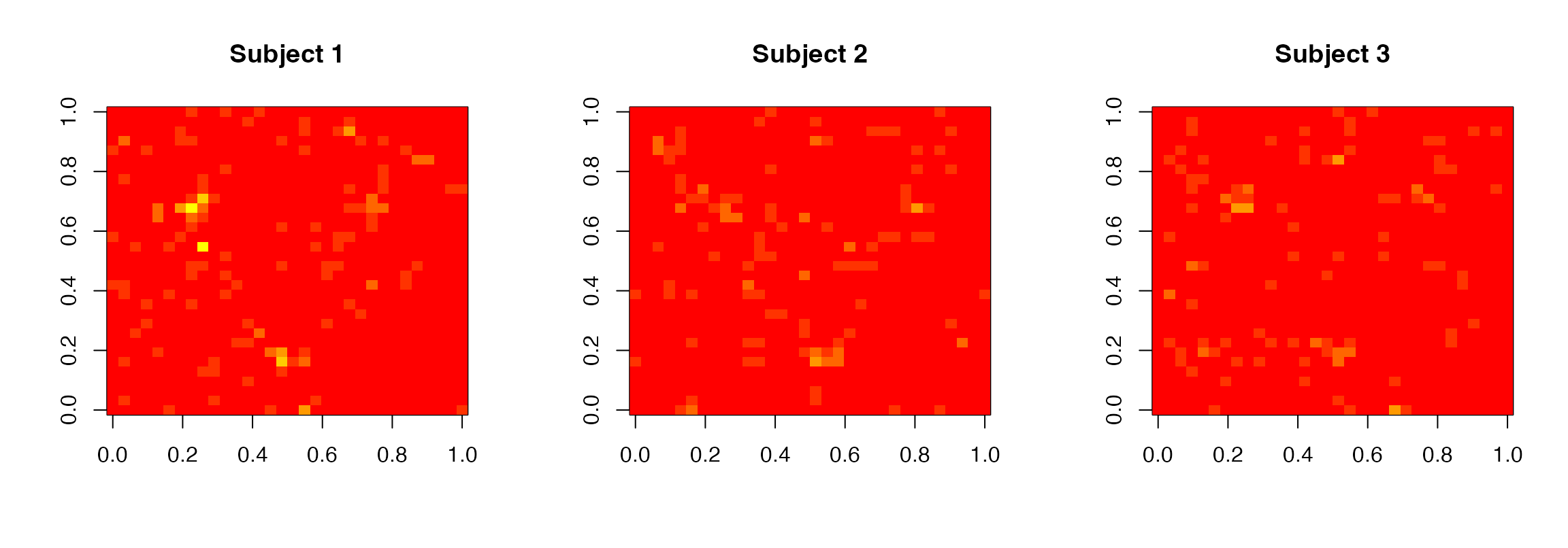
Posterior standardized regression coefficient images for the 3 subjects obtained by BHMSMA
Figure @ref(fig:PostCoef), obtained by the following code, shows the images of the posterior standardized regression coefficients for the 3 subjects.
As the true coefficients are known, we can compute the mean squared error (MSE) using the following code.
MSE <- c()
for (i in 1:n)
 MSE[i] <- sum((as.vector(truecoef[i,,]/glmmap$GLMCoefSE[i,,,2])
                - as.vector(postglmmap$GLMcoefposterior[i,,]))^2)
round(MSE,3)
## [1] 446.322 309.666 306.513In (Sanyal and Ferreira 2012), we show that our multi-subject methodology performs better than some existing methodologies in terms of MSE.
Posterior simulation and uncertainty estimation:
postsamples
In order to simulate observations from the posterior distribution of
the regression coefficients, the function postsamples can
be used. The type of analysis must be mentioned. The code below shows
its use.
Postsamp <- postsamples( nsample=50, n, grid, glmmap$GLMCoefStandardized[,,,k],
               wavecoefglmmap$WaveletCoefficientMatrix,  hyperest$hyperparam,
               pkljbar$pkljbar, "multi", seed=123)
names(Postsamp)
## [1] "samples" "postdiscovery"
dim(Postsamp$samples)## [1] 3 32 32 50
dim(Postsamp$postdiscovery)## [1] 3 32 32The argument nsample denotes the number of samples to be
drawn. We can see postsamples returns the posterior samples
and the probabilities of posterior discovery (Morris et al. 2011) for all the subjects.
Figure @ref(fig:PostDiscovery), obtained by the following code, shows
the posterior discovery images based on the above 50 samples for the 3
subjects.
par(mfrow=c(1,n), cex=1)
for(subject in 1:n)
  image(Postsamp$postdiscovery[subject,,], col=heat.colors(8),
   main=paste0("Subject ",subject))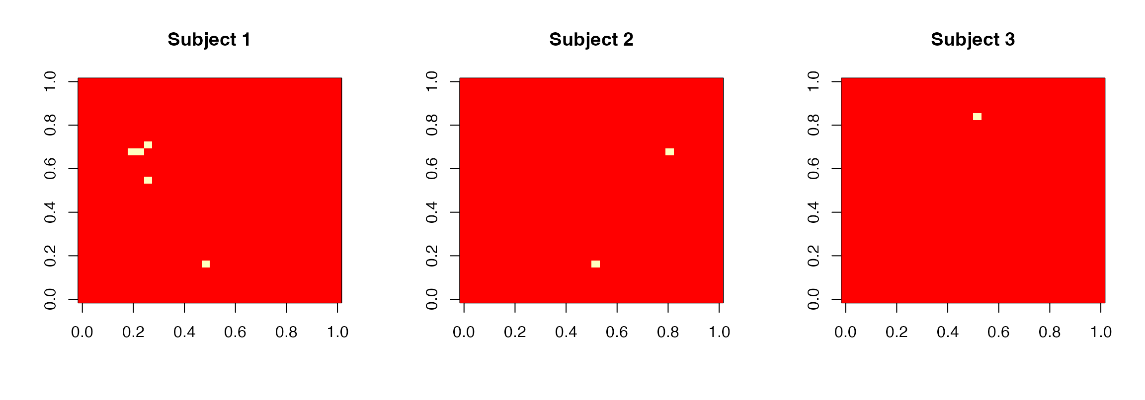
Posterior discovery images for the 3 subjects
From the posterior samples, the posterior standard deviations of the regression coefficients can be computed as follows.
postsd <- array(dim=c(n,grid,grid))
for(subject in 1:n)
 postsd[subject,,] <- apply(Postsamp$samples[subject,,,], 1:2, sd)
                             round(postsd[1,1:5,1:5],3)
## [,1] [,2] [,3] [,4] [,5]
## [1,] 0.466 0.496 0.471 0.677 0.677
## [2,] 0.655 0.737 0.531 0.677 0.687
## [3,] 0.657 0.465 0.472 0.435 0.656
## [4,] 0.656 0.702 0.470 0.581 0.597
## [5,] 0.571 0.468 0.417 0.532 0.508Posterior group estimates: postgroupglmcoef
Posterior group coefficients can be obtained by using the function
postgroupglmcoef as follows.
postgroup <- postgroupglmcoef( n, grid, glmmap$GLMCoefStandardized[,,,k],
                               postwavecoefglmmap$PostMeanWaveletCoef)
names(postgroup)
## [1] "groupcoef"
dim(postgroup$groupcoef)## [1] 32 32Figure @ref(fig:PostGroupCoef), obtained by the following code, shows the posterior group coefficient image for the simulated dataset.
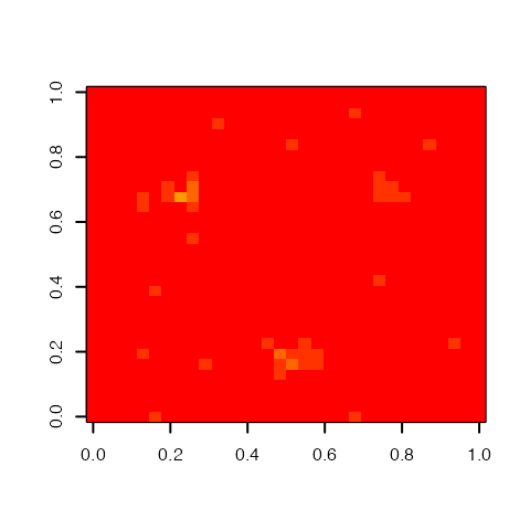
Posterior group regression coefficient image